Introduction

Avatria Convert is an eCommerce optimization tool that, among several capabilities, provides machine learning-derived product sorting that can be applied to product list pages (PLPs) or search engine result pages (SERPs). In other words, when a customer navigates to a category page, Convert will sort the items so that the most relevant results are at the top of the page.

Sort optimization tends to work well to drive conversion, revenue, and customer engagement—we recently observed a +30% increase in purchases and a +15% gain in clickthrough rate in an A/B test for a perfume retailer—but it’s also not unique in the field to observe certain cases where conversion metrics increase while average order value (AOV) or other revenue-based metrics decrease. This is not surprising: aside from some select industries, item price is generally inversely correlated with engagement and conversion.

This is a tricky issue. While driving conversion has numerous benefits outside of the revenue generated, most businesses will ultimately judge a tool by the effect it has on the bottom line. Resolving this potential conflict was the inspiration for our Data Science team to develop ranking models that could balance the two core objectives for any eCommerce site: conversion and revenue.

We wanted to use this blog post to share the results of our research into this topic. The first half of the post will share a high-level overview of what we did and what we found, while the second half will provide detailed explanations for the more technically minded.

The Problem

As mentioned previously, when it comes to balancing conversion and revenue, there is no free lunch: the two concepts are fundamentally at odds. The lower the relative cost of an item, the more likely an interested user is to buy it (see: coupons). On the flip side, any of us can think of countless cases where we’ve decided not to buy something we otherwise wanted because the price was too high.

When it comes to relevance and product ordering, the issues gets more complicated. It’s difficult to gauge whether or not users would have clicked on or purchased items had they been ordered differently. There are a lot of factors that impact the likelihood a customer will interact with a given product—its position, the customer’s patience, list pagination, the quality of other products presented, the list goes on. 

But we do know that users are vastly biased towards items that come ranked at the top of a list. This is true across all sites and industries, as is exemplified in the chart below.

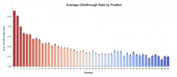
_{Average clicks per position for a Convert customer’s training data comprised of PLP and SERP query result sets. Position bias shows that users are almost three times as likely to click on items in positions one or two than in positions 15+.}

As such, in order to maximize revenue, we’ll have to make a tradeoff. By moving more expensive items towards the top of a PLP or SERP, we increase the probability of those items being purchased, and the overall revenue generated by the list. However, by moving less desirable items into these key positions, we may end up decreasing overall engagement and conversion rates. The challenge for the data science team, then, was to find the happy medium.

Methods

After studying other eCommerce companies’ approaches to this problem, we decided to evaluate two different methods for optimizing revenue. These methods were broadly similar in that they relied on a two-step process, where our base relevance model (which does does not consider product price) was augmented with a post-processing step to incorporate price.

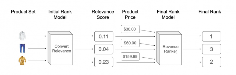
_{An example of the two-step revenue-aware rank model flow.}

These two approaches were as follows:

• A relevance-revenue hybrid (RRH) approach whereby we blended the relevance model output with a sort-ordering by price.

• An expected revenue (ER) approach whereby we sorted items by price multiplied by the predicted probability of purchase.

Relevance-Revenue Hybrid Model

Our inspiration for the RRH approach came from Rocket Travel’s popular blog posts on learning to rank hotel listings. For this method, we generated two sets of rankings: the product set ordered by relevance score, and the product set ordered by price. To oversimplify matters, we then applied a weighting to each ranking, created a combined score based on the weighted scores, and re-ranked the product set according to the combined RRH score.

For example, here’s what this might look like for a five-product list, using a weighting schema of 50% Relevance / 50% Price.

_{*In the above example, the highest ranked product is 5, the second ranked product is 4, etc.}

The biggest question with the RRH method is to figuring out the optimal weighting to give relevance (α) vs. price (1-α). In our research we experimented with three different weighting schemas to help us understand how great the relevance tradeoff would end up being in practice. The weightings we experimented with were:

• α = 0.9 (90% Relevance / 10% Price)

• α = 0.5 (50% Relevance / 50% Price)

• α = 0.2 (20% Relevance / 80% Price)

Expected Revenue Model

Etsy’s 2019 paper, “Joint Optimization of Profit and Relevance for Recommendation Systems in E-commerce,” was the major starting point for us in developing our expected revenue model. We liked the simplicity and clarity of this method, as it took the predicted purchase probabilities output by a classifier model and multiplied them by a price function, g(x). We could then simply sort by this expected revenue value.

We tested several versions of the ER model by modifying the price function. The two most promising price functions we tested were the identity function, where g(x) = price, and a log function, where g(x) = ln(price). We decided to try out different price functions because we were worried about price skewing the ER model’s output by overpower relevance in the model. 

If you’d like to get into the nitty-gritty of either approach, please see the Appendix section at the end of the article.

Evaluation

We’re about to get into a detailed discussion of our evaluation methodology that can get pretty wonky. If math isn’t your forte, feel free to skip ahead to the Final Choice section below.

We compared each method on datasets from three Convert customers using a variety of both relevance and revenue-based metrics. The evaluation metrics used were as follows:

• NDCG@k: relevance measure. This is the traditional measure of how well-sorted a list is according to relevance scores.

• AvgPrice@k: revenue measure. The average price among items in the top-k positions.

• NDCP@k: revenue measure. This is a play off of NDCG, but where the concept of "relevance” is swapped with price. It measures how well sorted a list is with respect to price (descending).

Comparing Rank Methods: ECDF Area-Under-Curve Reduction

To evaluate the impact of incorporating price into model rankings, the data science team found empirical cumulative distribution function (ECDF) charts extremely useful. These charts plot what percentage of all product sets have a model score under a given metric threshold. For example, in the graphic at the end of this section, approximately 87% of all product sets in the baseline dataset had an NDCG below 0.5. For the rank model, on the other hand, only a hair above 50% of product sets had an NDCG below that mark. This indicates that the model is producing more relevant rankings, as a larger share of all product sets have higher relevance scores.

As such, an ideal ECDF plot would look like a long, flat valley that rises dramatically to a narrow peak close to 1.0, indicating that most product sets have high scores (see example drawing below). If drawing an ECDF plot for a relevance metric (like NDCG), that narrow peak would tell us that the model has effectively optimized for relevance; if using a price metric (like NDCP), a narrow peak would tell us that the model has effectively sorted the most expensive products at the top of the list.

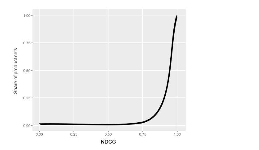
_{Example of what an ideal ECDF curve would look like. Unfortunately, you’re unlikely to encounter one of these in the wild.}

By drawing ECDF curves for multiple models on the same plot, we can easily visualize the tradeoff between relevance and revenue. In fact, we can even quantify it by calculating the area-under-curve (AUC). Because we want the area under the curve to be as small possible for any given metric, we can compare the AUC values of different models, telling us the relative improvement between them.

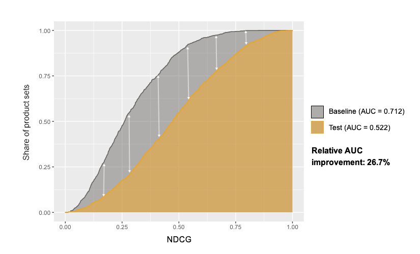
_{Illustration of a rank model’s NDCG ECDF and its reduction in AUC (the difference between grey and orange curves) over the NDCG of the baseline ranking. In this case, the rank model has reduced the AUC by 26.7%.}

Results

As expected, our research confirmed our suspicions about the tradeoff between relevance and price. The below charts shows how different versions of our relevance-revenue hybrid model performed, according to NDCG and AvgPrice. We plotted all three versions of the RRH model against both a baseline figure (the blue line), and our standard relevance model (the orange line).

The most aggressive of the RRH permutations we experimented with, the 20% relevance / 80% price hybrid, is the green line below. We can clearly see that this model has the highest proportion of product sets below each relevance benchmark, and thus the largest AUC. However, the second chart shows us that it has effectively raised the average price of products in the first 20 positions. This same tradeoff applied to the ER ranker as well.

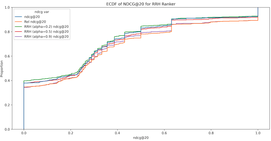
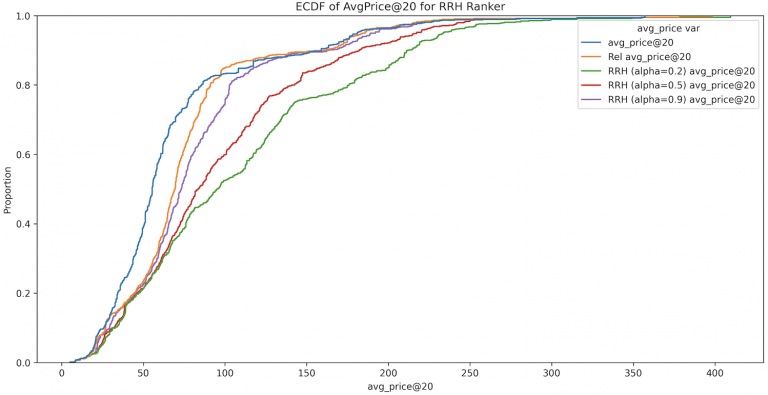
_{(Top) NDCG@20 ECDF of the RRH Ranker for Customer 1. The ECDF curves of the RRH rankers lie between that of the holdout set (blue curve) and the baseline relevance ranker (orange curve), illustrating the tradeoff between relevance and revenue. (Bottom) AvgPrice@20 ECDF for the RRH ranker for Customer 1.}

To help us compare the relative gain and loss of each model, we created the table below, which shows how each model performed across evaluation metrics, as compared to the baseline holdout set. We can see that while the RRH model’s NDCG gain dropped from +5.70% in the base ranker to +4.50%, it achieved a +33.77% improvement in NDCP, as compared to the base model’s +7.58%. Needless to say, trading a small amount of relevance for that much revenue potential is well worth it. The data science team’s goal, then, is to pick the method that provides the least sacrifice with the most upside.

_{The AUC under various metrics’ ECDF curves and their corresponding percentage improvement over the holdout set for Customer 1. The purchase classifier model causes a leftward shift in the AvgPrice EDCG – evidence that Customer 1’s customers prefer to purchase less expensive items.}

Final choice

In an effort to simplify the decision between RRH and ER ranker metrics, we placed each ranker’s performance on each metric into either 1st, 2nd, or 3rd place across the three customers included in the experiment. Overall the RRH (α = 0.9) ranker comes in first place for NDCG for two customers and 3rd place for another customer, so the RRH ranker gets 1.7th place for NDCG. Our full-table is below.

_{Comparison across NDCG, Revenue, NDCP, and AvgPrice metrics across RRH and two types of ER rankers.}

Our best-in-class revenue ranker was the expected revenue ranker, but closely trailed by RRH (α = 0.9). Given the closeness of the two’s performance, we decided to follow the RRH approach as our standard revenue optimization strategy for a few reasons.

• Tune-ability of the revenue-relevance tradeoff parameter. The data science team can easily render scatterplots of NDCG vs AvgPrice for different weightings of revenue vs. relevance and then pick the best performing value for each customer. 

• Direct interpretability of the revenue-relevance tradeoff parameter.

• Extensibility to other ranking objectives. This study only analyzed the combination of 

  price and relevance, but the rank product algorithm lets us extend the RRH concept to any customer’s objective, such as profit margin, inventory level, or newness. In fact, we could even create more complicated blends, such as a model that considers two or more additional objectives.

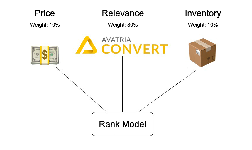
_{The extensibility of the rank product algorithm. Not only can we blend product price with Convert’s relevance ranking models, but we could add any number of other product features to help sort items according to our customers’ needs, e.g. inventory, using a simple weight normalization scheme.}

We hope you enjoyed this deep-dive into Convert Engineering! If you are curious about trying Convert, get in touch for a free-trial. We can run a 30-day free A/B test for your B2B or B2C eCommerce site so that you can start getting improved list-attributed engagement and revenue KPIs!

Appendix

Relevance-Revenue Hybrid Model

Rocket Travel first proposes an expected revenue ranking based upon “querywise softmax probabilities.” This means that we would take the model scores predicted by a lambdarank-objective ranking model, which are continuous, and transform them into “probabilities” between (0, 1):

The querywise softmax probabilities would then be multiplied by revenue (or profit, if that data is available) and the final ranking would be a sort-ordering of items by decreasing expected revenue or profit.

The problem with using querywise probability scores like this are twofold:

1. Unlike in hotel listings, generic eCommerce customers may purchase multiple items during a single query session. Since groupwise probability scores must sum to 1 across the items returned as part of the query, if three items , the best possible “probability” distribution would assign each item a probability of only 0.33, not 1.

2. Probabilities and price are on vastly different scales. Convert customers range from B2B companies who sell inexpensive items in bulk to luxury perfume distributors selling $400 bottles of perfume. So price can very quickly “dominate” any ranking by probability scores even under modest amounts of within-query price variance.

Rocket Travel offered a solution to the second issue by using a rank product, similar to a geometric mean, which is what led us to the approach we followed:

To recap, that approach is as follows: 

1. Convert’s relevance ranking models default to a graded relevance labeling scheme where product impressions begin with a score of 0, clicked items receive a 1, items added to the customer’s cart receive a 2, checkouts receive a 3, and purchased items receive a maximum score of 4.

2. Next, we train a ranking model using the LambdaRank objective with the popular 

   “unbiased” loss function modification. LambdaRank loss is defined across pairs of differentially-relevant items within groups of items we refer to as query result sets.

3. Run all query result sets through the relevance model, and then apply the rank product procedure using the output model scores alongisde each item’s price. To reiterate, the rank of product i can be expressed using the following formula:

ranki = rank(rank(f(xi))αrank(ri)1-α)

where f(x_i) is the base relevance ranking model’s output relevance score for the product, r_i is the price of the product, and α is the objective tradeoff weight. For our experiments we set a conservative α=0.9, but also examined the performance curves for the values α=0.2 and α=0.5 as well.

As a future area of research, the data science team may experiment with different discretization strategies and start grouping similar scores or prices into the same rank. For example, two consecutive items whose prices differ by $100 would be treated differently than two items whose prices differ by only $0.50. Similarly, if the most relevant item in the list is given a score of 2.7 by the model and the next-most relevant item only receives a score of 0.1, an alternative ranking function might be able to better account for this scale difference rather than assigning ranks 1 and 2.

Expected Revenue Model

Etsy’s paper, on the other hand, actually attempts to directly maximize a two-part objective function combining relevance and expected revenue (or in the case of the paper, expected profit):

We refer to this as the “Etsy objective.” Its objective function is wonderful for its simplicity and directness in expressing the relevance/revenue tradeoff. But the authors provide no insights into how to choose c. The benefit of α is that it’s scaled within (0, 1), but the choice of c will vary depending on the price variance of every individual customer’s product catalogs. Further, the fact that expected revenue is so easily “hacked” made the data science team nervous: it could be very easy for a model to become trapped at the obvious local maximum of the Etsy objective—the classifier that predicts “every product will be purchased,” thus achieving maximum “expected revenue.” While we could create custom gradient, hessian, and metric functions to maximize the Etsy objective with a tool like LightGBM (instead of via linear programming methods as suggested by the paper’s authors), this lack of intuition as how to set c ahead of time made the data science team hesitant to directly maximize the Etsy objective.

Despite our concerns regarding maximizing the Etsy objective, the Convert data science team did evaluate a second model tested in the Etsy paper, the expected revenue ranker using a weighted logistic loss. The most apparent drawback of the RRH approach is that it’s divorced from the concept of expected revenue entirely, so the data science team saw it fit to compare a relevance-based ranker and this proposed expected revenue-based ranker.

Our methodology was as follows:

1. In order to build a classifier, we simply re-label purchased items to y=1 and non-urchased items to y=-1.

2. Train a classifier using a weighted loss function. The loss is increased for the positive class (purchased items) by the item’s price so that the classifier suffers a larger penalty for incorrectly classifying expensive purchases than cheap purchases.

   $$\mathcal{L} = \sum_{i | y_{i} = 1}\text{price}_{i}\log(1 + e^{-y_{i}(\theta^{T} x_{i})}) + \sum_{j | y_{j} = -1} \log(1 + e^{-y_{i}(\theta^{T} x_{i})})$$

   1. The training data will be severely imbalanced due to the fact that queries resulting in purchases are relatively rare. Further, within each query result set only a small minority of items in a list of product impressions are typically purchased. To combat this imbalance, we removed queries from the training dataset that did not contain any positive class instances. The holdout set was not similarly filtered, but contained queries that did and did not contain a purchase.

3. Rank items within each query according to predicted model probability multiplied by price: p̂_ir_i, or expected revenue, descending. We can think of an expected revenue ranker as f(x_i)g(r_i), where f(x_i) is the predicted probability of purchase output from the classifier for product i, and g(r_i) is just some function of the product’s price.

   1. To lessen the impact of large price outliers, we also used g(r_i) = ln(r_i), so that the final ranking is according to p̂_iln(r_i).